Theory
The solution process begins by evaluating the two continuous analytical catenary equations for each element based on \(l\) and \(h\) values obtained through node displacement relationships. An element is defined as the component connecting two adjacent nodes together. Once the element fairlead (\(H\), \(V\) ) and anchor (\(H_a\), \(V_a\)) values are known at the element level, the forces are transformed from the local \(x_i z_i\) frame into the global \(XYZ\) coordinate system. The force contribution at each element’s anchor and fairlead is added to the corresponding node it attaches to.
The force-balance equation is evaluated for each node, as follows:
Node forces are found based on the connectivity geometry between element and external forces applied at the boundary conditions. This is initiated by defining a series of \(\mathcal{F}_i\) local frames at the origin in which the individual line elements are expressed in. Frame \(\mathcal{F}_0\) is an arbitrary global axis, but it is usually observed as the vessel reference origin.
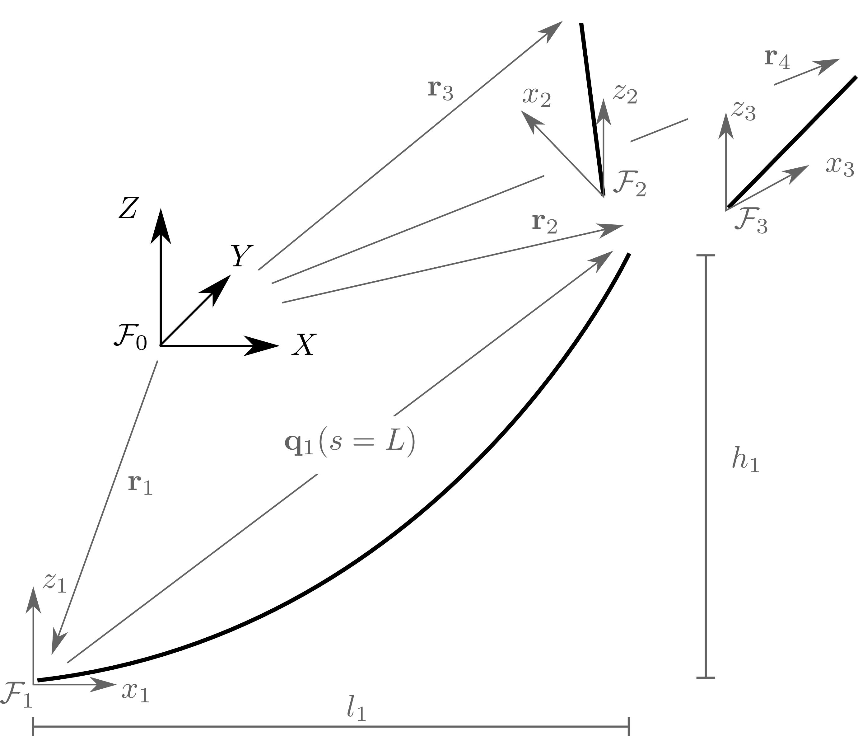
Fig. 2
Note
Simplistic way to think of MAP++’s dichotomy between nodes and elements: Nodes define the force at connection points. Elements define the mooring geometry.
Clearly, this process requires two distinct sets of equations, one of which must be solved within the other routine, to find the static cable configuration. The first set of equations are the force{balance relationships in three directions for each node; the second set of equations are the catenary functions proportional to the number of elements. Interactions between solves is captured in the flowchart below to summarize the solve procedure. This method was first proposed in [4].
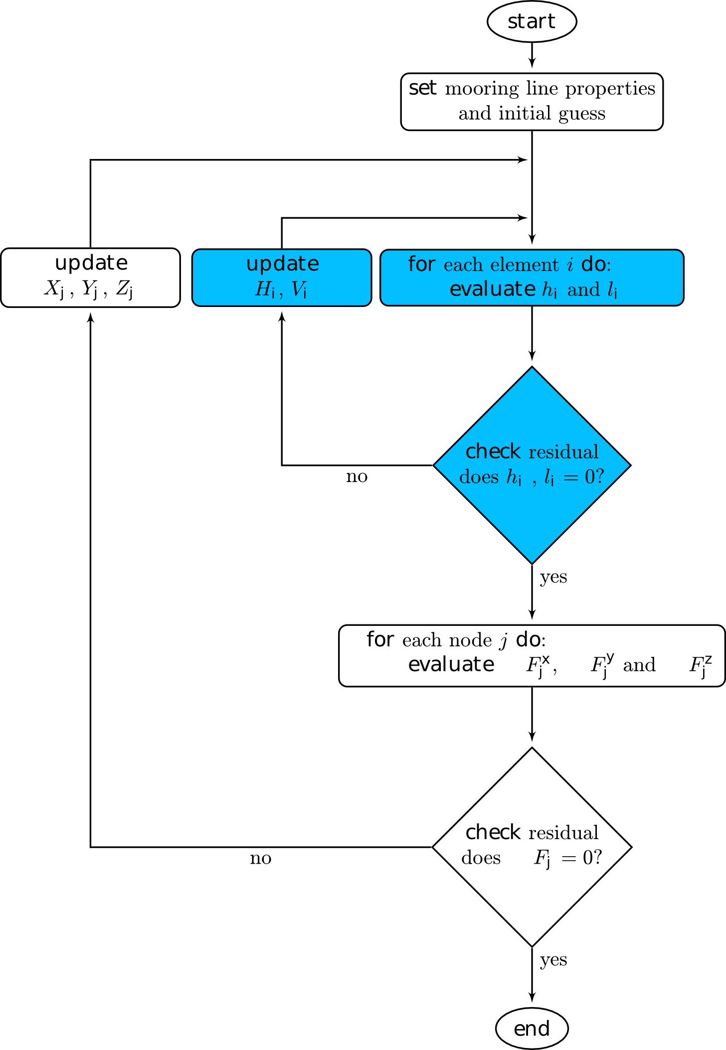
Fig. 3
Line Theory
Free–Hanging Line
The equations used to describe the shape of a suspended chain illustrated in Fig. 4 have been derived in numerous works [1]. For completeness, a summary of the governing equations used inside the MSQS model are presented. Given a set of line properties, the line geometry can be expressed as a function of the forces exerted at the end of the line:
where:
and \(x\) and \(z\) are coordinate axes in the local (element) frame, Fig. 2. The following substitution can be made for \(V_a\) in the above equations:
which simply states the decrease in the vertical anchor force component is proportional to the mass of the suspended line. The equations for \(x(s)\) and \(z(s)\) both describe the catenary profile provided all entries on the right side of the equations are known. However, in practice, the force terms \(H\) and \(V\) are sought, and the known entity is the fairlead excursion dimensions, \(l\) and \(l\). In this case, the forces \(H\) and \(V\) are found by simultaneously solving the following two equations:
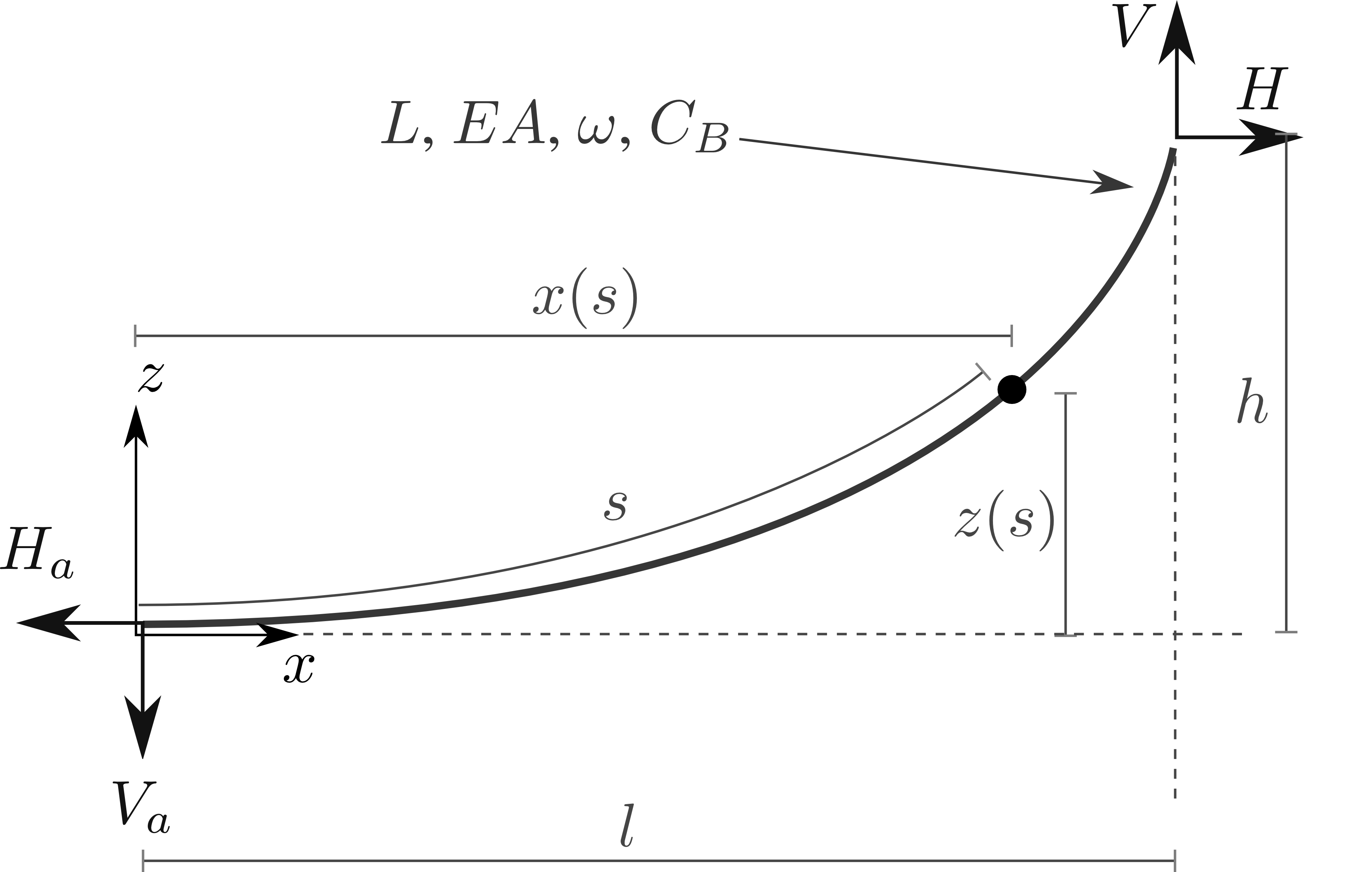
Fig. 4
Line Touching the Bottom
The solution for the line in contact with a bottom boundary is found by continuing \(x(s)\) and \(z(s)\) beyond the seabed touch–down point \(s=L_{B}\). Integration constants are added to ensure continuity of boundary conditions between equations:
where \(\lambda\) is:
Between the range \(0\leq s \leq L_{B}\), the vertical height is zero since the line is resting on the seabed and forces can only occur parallel to the horizontal plane. This produces:
The equations above produce the mooring line profile as a function of \(s\). Ideally, a closed–form solution for \(l\) and \(h\) is sought to permit simultaneous solves for \(H\) and \(V\), analogous to the freely–hanging chase in the previous section. This is obtained by substituting \(s=L\) to give:
Finally, a useful quantity that is often evaluated is the tension as a function of \(s\) along the line. This is given using:
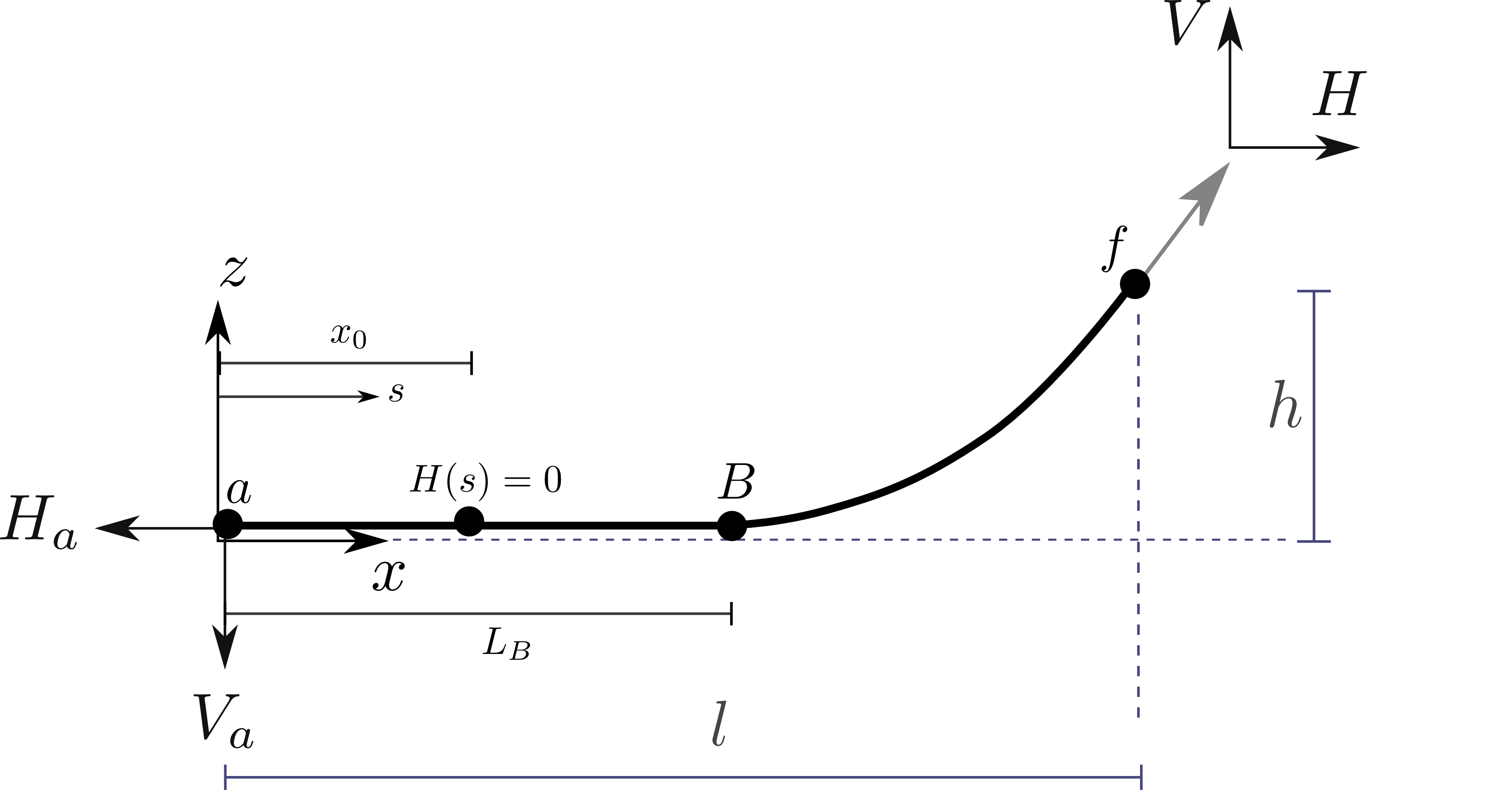
Fig. 5
Vessel
Reference Origin
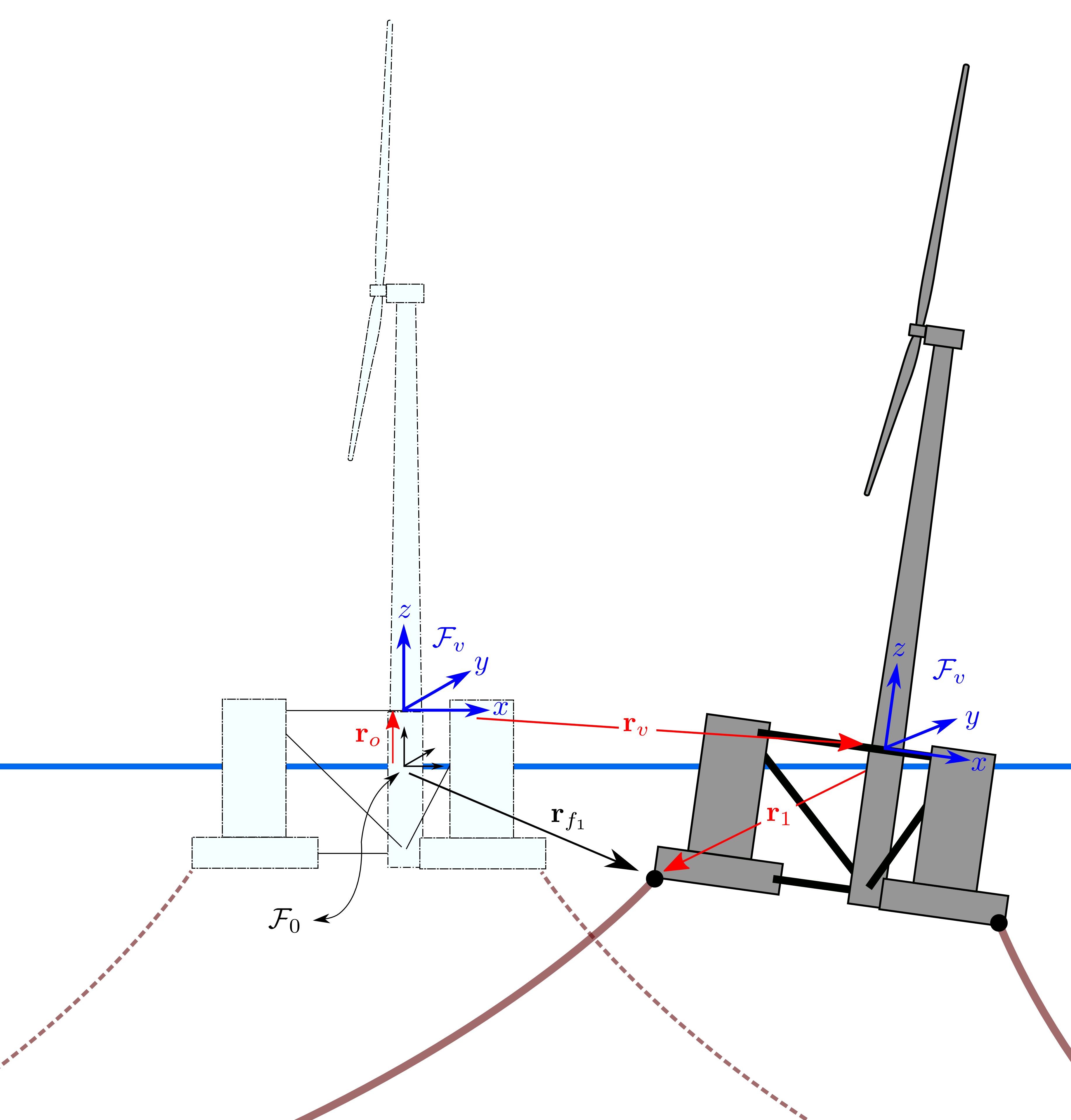
Fig. 6