Python Example
Static Configuration
This example will be run against the baseline input file.
The water depth is \(350\) meters.
The space preceeding the repeat 120 240 solver option flag is removed to enable duplication of the mooring geometry twice with \(120^\circ\) and \(240^\circ\) offsets about the \(Z\) axis.
#! /usr/bin/env python
# -*- coding: utf-8 -*-

'''
Copyright (C) 2015
map[dot]plus[dot]plus[dot]help[at]gmail
License: http://www.apache.org/licenses/LICENSE-2.0
'''

from mapsys import *
import matplotlib.pyplot as plt
from mpl_toolkits.mplot3d import Axes3D
import numpy as np
np.set_printoptions(precision=2)
np.set_printoptions(suppress=True)


if __name__ == '__main__':
    mooring_1 = Map()

    mooring_1.map_set_sea_depth(350)      # m
    mooring_1.map_set_gravity(9.81)       # m/s^2
    mooring_1.map_set_sea_density(1025.0) # kg/m^3

    mooring_1.read_file("../test/baseline_2.map")
    mooring_1.summary_file('summary_file.txt')

    mooring_1.init( )

    epsilon = 1e-3 # finite difference epsilon
    K = mooring_1.linear(epsilon)
    print "\nLinearized stiffness matrix with 0.0 vessel displacement:\n"
    print np.array(K)

    surge = 5.0 # 5 meter surge displacements
    mooring_1.displace_vessel(surge,0,0,0,0,0)
    mooring_1.update_states(0.0,0)

    K = mooring_1.linear(epsilon)
    print "\nLinearized stiffness matrix with %2.2f surge vessel displacement:\n"%(surge)
    print np.array(K)

    # We need to call update states after linearization to find the equilibrium
    mooring_1.update_states(0.0,0)

    line_number = 0
    H,V = mooring_1.get_fairlead_force_2d(line_number)
    print "Line %d: H = %2.2f [N]  V = %2.2f [N]"%(line_number, H, V)

    fx,fy,fz = mooring_1.get_fairlead_force_3d(line_number)
    print "Line %d: Fx = %2.2f [N]  Fy = %2.2f [N]  Fz = %2.2f [N]\n"%(line_number, fx, fy, fz)

    print "These values come from the output buffer as defined in the 'LINE PROPERTIES' portion of the input file"
    print "Labels : ", mooring_1.get_output_labels()[0:6]
    print "Units  : ", mooring_1.get_output_units()[0:6]
    v = mooring_1.get_output_buffer()[0:6]
    print "Values : ", ["{0:0.2f}".format(i) for i in v]

    fig = plt.figure()
    ax = Axes3D(fig)
    num_points = 20
    for i in range(0,mooring_1.size_lines()):
        x = mooring_1.plot_x(i, num_points)
        y = mooring_1.plot_y(i, num_points)
        z = mooring_1.plot_z(i, num_points)
        ax.plot(x,y,z,'b-')

    ax.set_xlabel('X [m]')
    ax.set_ylabel('Y [m]')
    ax.set_zlabel('Z [m]')

    plt.show()

    mooring_1.end( )
Output
Two outputs are produced executing the stript above. Information explicitly requested is printed to the command line:
MAP++ (Mooring Analysis Program++) Ver. 1.20.10 Mar-22-2016
MAP++ environment properties (set externally)...
    Gravity constant          [m/s^2]  : 9.81
    Sea density               [kg/m^3] : 1025.00
    Water depth               [m]      : 350.00
    Vessel reference position [m]      : 0.00 , 0.00 , 0.00

Linearized stiffness matrix with 0.0 vessel displacement:

[[  1.99e+04  -3.78e-03   5.19e-03  -4.89e-02  -2.00e+05  -1.77e-02]
 [  1.18e-03   1.99e+04  -1.06e-02   2.00e+05   3.50e-02  -6.17e-01]
 [  2.49e-03  -1.01e-03   2.27e+04   2.21e-03   2.23e-01  -2.12e-01]
 [  1.95e-03   2.00e+05  -7.14e-03   2.17e+08   1.10e-02  -5.23e+01]
 [ -2.00e+05   3.33e-04   4.85e-01  -4.89e-02   2.17e+08  -2.19e-02]
 [  8.83e-04  -5.59e-01   1.12e-03  -8.53e+01  -7.90e-02   1.41e+08]]

Linearized stiffness matrix with 5.00 surge vessel displacement:

[[  1.96e+04  -2.58e-05   1.17e+03   9.61e-03  -2.15e+05  -1.67e-01]
 [ -4.57e-04   2.07e+04   1.41e-03   1.81e+05  -5.24e-02   1.72e+03]
 [  1.17e+03  -3.32e-04   2.32e+04  -5.38e-03  -1.19e+04   1.12e-03]
 [  1.05e-03   2.00e+05   1.51e-03   2.17e+08   4.25e-02  -5.21e+01]
 [ -2.00e+05  -8.91e-05   4.79e-01   5.43e-03   2.17e+08   6.60e-02]
 [  2.10e-03  -5.60e-01   5.77e-03  -8.52e+01   1.07e-01   1.41e+08]]
Line 0: H = 597513.33 [N]  V = 1143438.75 [N]
Line 0: Fx = -597513.33 [N]  Fy = -0.00 [N]  Fz = 1143438.75 [N]

These values come from the output buffer as defined in the 'LINE PROPERTIES' portion of the input file
Labels :  ['l[1]', 'alpha[1]', 'T[2]', 'l[4]', 'alpha[4]', 'T[5]']
Units  :  ['[m]', '[rad]', '[N]', '[m]', '[rad]', '[N]']
Values :  ['338.18', '1.07', '711942.60', '338.18', '1.07', '711942.39']
A figure is also produced to show the mooring geometry with a \(5\) meter vessel offset:
Note
The default units for the linearized stiffness matrix are [N/m], [N/rad], [Nm/m], and [Nm/rad]. See the section on the linearized stiffness matrix in the FAQ for more information.
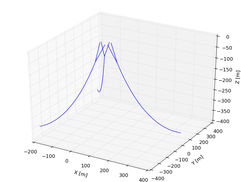
Fig. 7
Time-Marching for Dynamics Simulation
#! /usr/bin/env python
# -*- coding: utf-8 -*-

'''
Copyright (C) 2015
map[dot]plus[dot]plus[dot]help[at]gmail
License: http://www.apache.org/licenses/LICENSE-2.0
'''

from mapsys import *
import math
import matplotlib.pyplot as plt
from mpl_toolkits.mplot3d import Axes3D
import matplotlib.ticker as mtick
from matplotlib import rcParams
import numpy as np
np.set_printoptions(precision=2)
np.set_printoptions(suppress=True)
rcParams.update({'figure.autolayout': True})


# user function to plot the mooring profile and footprint
def plot_mooring_system(mooring_data):
    # plot the mooring profile
    fig = plt.figure(1)
    ax = Axes3D(fig)
    colors = ['b','g','r','c']
    for i in xrange(mooring_data.size_lines()):
        x = mooring_data.plot_x( i, 20 ) # i is the the line number, and 20 is the number of points plotted on the line
        y = mooring_data.plot_y( i, 20)
        z = mooring_data.plot_z( i, 20)
        ax.plot(x,y,z,colors[i]+'-')
    ax.set_xlabel('X [m]')
    ax.set_ylabel('Y [m]')
    ax.set_zlabel('Z [m]')


def start():
    """
    Step 1) First initialize an instance of a mooring system

    Step 2) Assume that (X, Y, Z, phi, theta, psi) are the translation and rotation displacement of the vessel.
    These displacements are fed into MAP as an argument to displace the fairlead. With the fairlead(s)
    rigidly connected to the vessel, the (X, Y, Z, phi, theta, psi) directly manifests into the fairlead
    position in the global frame.

    For the time being, assume a sinusoidal displacement of the vessel

    Step 3) This for-loop emulates the time-stepping procedure. You want to loop through the length of
    the arrays (X,Y,Z,phi,theta,psi) to retrieve the fairlead force

    Step 4) update the MAP state. The arguments in displace_vessel are the displace displacements and rotations about the reference origin.
    In this case, the reference origin is (0,0,0).
    They can be set to a different potision using a run-time argument (this is an advanced feature).

    Step 5) get the fairlead tension. The get_fairlead_force_3d returns the fairlead force in
    X, Y Z coordinates. This must be called at each time-step, and then stored into an array. We append
    the empty lists created on lines 84-88.

    .. Note::

       MAP does *NOT* return the mooring restoring moment, The user must calculate this
       themself using the cross-product between the WEC reference origin and the mooring attached
       point, i.e.,

       :math:`\mathbf{Moment} = \mathbf{r} \times \mathbf{F}`
    """

    # Step 1
    mooring = Map()
    mooring.map_set_sea_depth(120)        # m
    mooring.map_set_gravity(9.81)         # m/s^2
    mooring.map_set_sea_density(1020.0)   # kg/m^2
    mooring.read_file('../test/baseline_1.map')   # input file
    mooring.summary_file('summary_file.sum.txt') # output summary file name at the conclusion of initialization

    mooring.init()                # solve the cable equilibrium profile
    plot_mooring_system(mooring) # Optional: call the user function to illustrate the mooring equilibrium profile


    # initialize list to zero (this is artificial. This would be prescribed the by vessel program)
    X,Y,Z,phi,theta,psi = ([0.0 for i in xrange(500)] for _ in xrange(6))
    time = []

    # variable to specify the amplitude of surge oscillation and period factor
    dt = 0.1
    amplitude = 10.0

    # prescribe artificial surge and pitch displacement. Again, this should be supplied based on the WEC motion or from time-marching routine
    for i in xrange(len(X)):
        time.append(i*dt)
        X[i] = (amplitude)*(math.sin(i*0.05))
        theta[i] = (amplitude)*(math.sin(i*0.025))

    # create an empty list of the line tension. We will store result from MAP in these lists
    line1_fx, line1_fy, line1_fz = ([] for _ in xrange(3))
    line2_fx, line2_fy, line2_fz = ([] for _ in xrange(3))
    line3_fx, line3_fy, line3_fz = ([] for _ in xrange(3))
    line4_fx, line4_fy, line4_fz = ([] for _ in xrange(3))

    # Step 3) Time marching
    for i in xrange(len(X)):
        # Step 4)

        # displace the vessel, X,Y,X are in units of m, and phi, theta, psi are in units of degrees
        mooring.displace_vessel(X[i], Y[i], Z[i], phi[i], theta[i], psi[i])

        # first argument is the current time. Second argument is the coupling interval (used in FAST)
        mooring.update_states(time[i], 0)

        # Step 5)
        # line 1 tensions in X, Y and Z. Note that python is indexed started at zero
        fx, fy, fz = mooring.get_fairlead_force_3d(0) # arugment is the line number
        line1_fx.append(fx)
        line1_fy.append(fy)
        line1_fz.append(fz)

        # line 2 tensions in X, Y and Z.
        fx, fy, fz = mooring.get_fairlead_force_3d(1)
        line2_fx.append(fx)
        line2_fy.append(fy)
        line2_fz.append(fz)

        # line 3 tensions in X, Y and Z.
        fx, fy, fz = mooring.get_fairlead_force_3d(2)
        line3_fx.append(fx)
        line3_fy.append(fy)
        line3_fz.append(fz)

        # line 4 tensions in X, Y and Z.
        fx, fy, fz = mooring.get_fairlead_force_3d(3)
        line4_fx.append(fx)
        line4_fy.append(fy)
        line4_fz.append(fz)

    # Optional: plot the vessel displacement (surge=X and pitch=theta) as a function of time
    plt.figure(2)
    plt.plot(time,X,lw=2,label='Surge displacement')
    plt.plot(time,theta,lw=2,label='Pitch displacement')
    plt.title('Vessel Translation/Rotation')
    plt.ylabel('Amplitude [m,deg]')
    plt.xlabel('Time [sec]')
    plt.legend()

    # Optional: plot line tension time history
    plt.figure(3)
    ax=plt.subplot(3,1,1)
    plt.plot(time,line1_fx,label='Line 1')
    plt.plot(time,line2_fx,label='Line 2')
    plt.plot(time,line3_fx,label='Line 3')
    plt.plot(time,line4_fx,label='Line 4')
    ax.yaxis.set_major_formatter(mtick.FormatStrFormatter('%.2e'))
    plt.ylabel('X Fairlead Force [N]')
    plt.legend()

    ax = plt.subplot(3,1,2)
    ax.yaxis.set_major_formatter(mtick.FormatStrFormatter('%.2e'))
    plt.plot(time,line1_fy)
    plt.plot(time,line2_fy)
    plt.plot(time,line3_fy)
    plt.plot(time,line4_fy)
    plt.ylabel('Y Fairlead Force [N]')

    ax = plt.subplot(3,1,3)
    ax.yaxis.set_major_formatter(mtick.FormatStrFormatter('%.2e'))
    plt.plot(time,line1_fz)
    plt.plot(time,line2_fz)
    plt.plot(time,line3_fz)
    plt.plot(time,line4_fz)
    plt.ylabel('Z Fairlead Force [N]')
    plt.xlabel('Time [sec]')

    plt.show()

if __name__ == '__main__':
    start()
Output
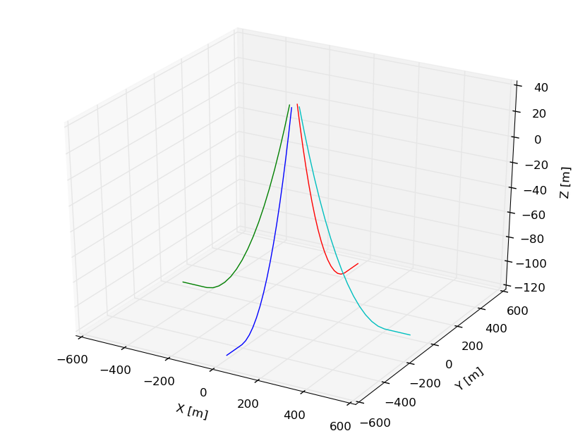
Fig. 8
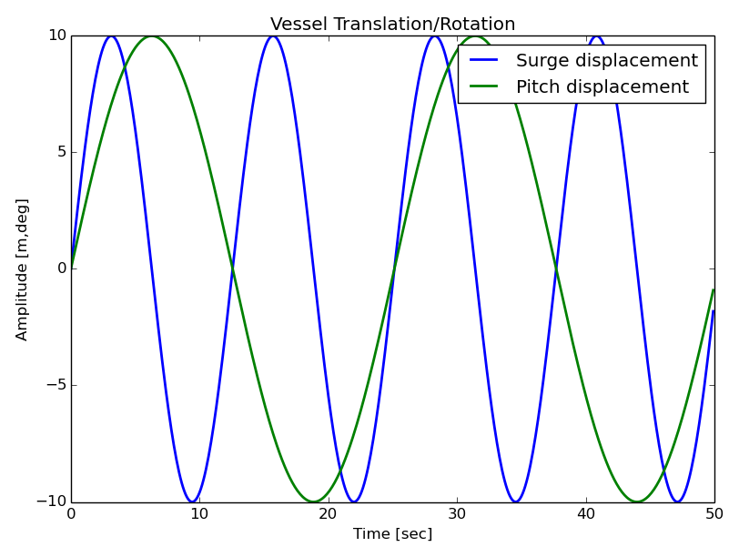
Fig. 9
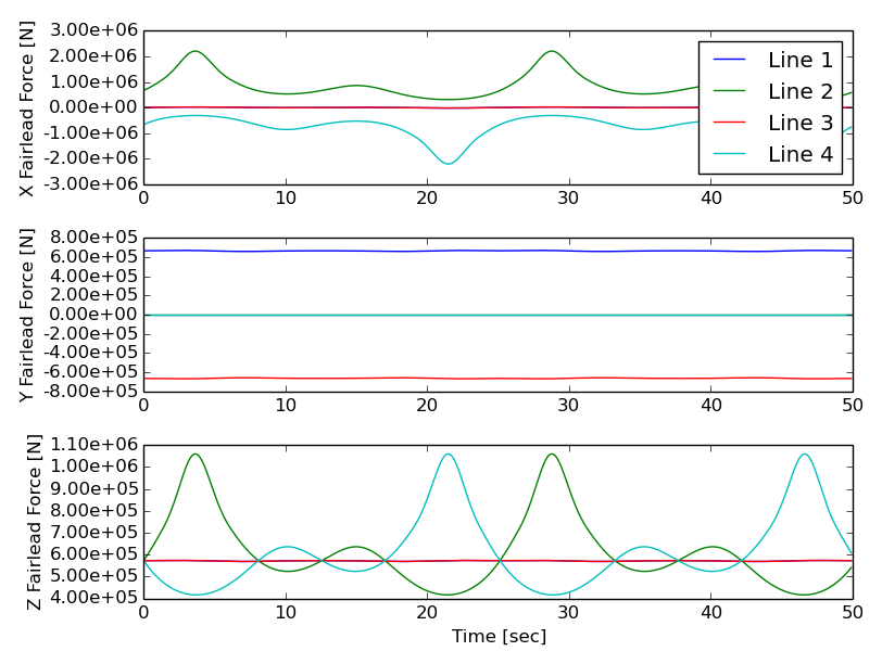
Fig. 10